1. Vibrating string

Idea of Fourier analysis comes from several physical questions. In this section, phenomena of the string vibration will be discussed.

Simple Harmonic Motion

Simple harmonic motion describes the behavior of the most basic oscillatory system. It contains a free spring with one side attached to a object which has mass of {M}, whose the other side fixed on the wall. To define the motion mathematically, we first define y(t) as the displacement of the Mass. According to the Hooker's law, the restoring force from the spring could be F=-ky(t). Applying Newton's law, we got
-ky(t)=my''(t)
where y''(t) is the second derivative of y with respect to t. This equation can be denoted as:
y''(t)+c\cdot y(t)=0
Such second order ordinary differential equation got general solution as:
y(t)=a\cos ct +b \sin ct
where a and b can be any real constants. But to determine the particular solution, two initial conditions must be imposed: the initial position y(0) and velocity y'(0) of the mass.
y(t)=y(0)\cos ct +\frac{y'(0)}{c} \sin ct
We can get two important observations of this formula: The first one is that the mathematical description of the motion involves the most fundamental trigonometric functions sine and cosine, which has connections with complex number by Euler's identity. Another observation is that the simple harmonic motion is determined as a function of time by two initial conditions: position and velocity.

Standing and traveling waves

Given the motion, how could we turn it into graphic representations? Here two solution will be introduced.

• Standing waves: Wavelike motions described as y=u(x,t) developing with t. We can also divide the function into two separate parts such as:
  u(x,t)=\phi (x) \psi(t)
  where \phi indicates the initial profile(t=0) while \psi indicates amplifying factor.

• Traveling waves: The initial profile F(x) will develop or be replaced by ct units.
  u(x,t)=F(x-ct)

1.1 Derivation of the wave equation

Turn our attention back to the string problem. Suppose there is a homogeneous string placed in the (x,y)-plane and stretched along x-axis from X=0 to X=L. The displacement of the string can be denoted as u(x,t). Our aim is to find the differential equation that governs the function.

We can divide the string into a large number N of masses or particles. Thus the coordinate of the n-th particle is x_n=nL/N.These particles all oscillates in vertical directions and link with the neighboring particles. Set y_n(t)=u(x,t) as the displacement of the mass and the string has constant density \rho>0, thus the mass of the n-th particle will be \rho h. We also set the tension of nearby particle as \Delta y \tau / h. According to Newton's Law
\rho h y''(t)=\frac{\tau}{h}(y_{n+1}+y_{n-1}-2\cdot y_{n})
Notice that when h->0
\frac{\tau}{h^2}(y_{n+1}+y_{n-1}-2\cdot y_{n}) =\frac{\partial^2 y}{\partial x^2}

We can get
\rho \frac{\partial^2 u}{\partial t^2}=\tau \frac{\partial^2 u}{\partial x^2}
or set c=\sqrt{\tau/\rho}
\frac{1}{c^2} \frac{\partial^2 u}{\partial t^2}= \frac{\partial^2 u}{\partial x^2}
This relation is known as the one-dimensional wave function. The coefficient c is called the velocity of the motion.

To simplify the equation, a scaling operation is required. We can then get:
\frac{\partial^2 U}{\partial T^2}= \frac{\partial^2 U}{\partial X^2}
where 0\leq x\leq \pi, with 0\leq t

1.2 Solution to the wave function

This equation can be solved by both standing waves and traveling waves.

Traveling waves

There is a crucial observation: If F is any twice differentiable function. Then u(x,t)=F(x+t) and u(x,t)=F(x-t) solve the wave equation.

Proof: Given the equation, we may get:
\frac{\partial^2 U}{\partial T^2}- \frac{\partial^2 U}{\partial X^2}=0

(\frac{\partial }{\partial T}+\frac{\partial }{\partial X})(\frac{\partial }{\partial T}-\frac{\partial }{\partial X})U=0

Set v=U_t-U_x
(\frac{\partial }{\partial T}+\frac{\partial }{\partial X})v=0
The solution of v could be
v(x,t)=h(x-t)
where h is a differentiable function. Then we try to solve
U_t-U_x=h(x-t)
This is a linear inhomogeneous first order equation with constant coefficients and could be solved as
U(x,t)=f(x-t)
where f'=h/2. Since h is once differentiable, f is then twice differentiable.

For v=U_t+U_x, vice versa

We also notice that wave equation is linear. This means if u(x,t) and v(x,t) are solutions, so as \alpha u(x,t)+\beta v(x,t) for any constant \alpha and \beta.
u(x,t)=F(x+t)+G(x-t)
Setting t=0 and u(x,0)=f(x) which gives the initial position,
F(x)+G(x)=f(x)
For initial velocity, define:
g(x)=\frac{\partial u}{\partial t}(x,0)

F'(x)-G'(x)=g(x)

Thus we get
F(x)=\frac{1}{2}[f(x)+\int_0^xg(y)dy]+C_1
Similarly,
G(x)=\frac{1}{2}[f(x)-\int_0^xg(y)dy]+C_2
Since F(x)+G(x)=f(x), we can get C_1+C_2=0, and the final solution (d' Alembert's formula) of the wave equation
u(x,t)=\frac{1}{2}[f(x+t)+f(x-t)]+\frac{1}{2}\int_{x-t}^{x+t}g(y)dy

Standing waves

A procedure called "separation of variables" works well when dealing with standing waves.
u(x,t)=\phi (x) \psi(t)
We first find special solution from the equation above which divide the function into a position part \phi and amplitude part \psi. Then by the linearity of the wave function, we may get a general solution of it. Take that equation into wave function, we get
\phi(x)\psi ''(t)=\phi ''(x)\psi(t)
or we set they both equal to a constant \lambda
\frac{\phi (x)}{\phi'' (x)}=\frac{\psi (t)}{\psi'' (t)}=\lambda
Thus the wave equation has such a form
\begin{cases}
\psi(t)-\lambda\psi''(t)=0 \\
\phi(x)-\lambda\phi''(x)=0
\end{cases}
The key observation is that these two equations both have the form of simple harmonic motion, they thus have the solution as
\begin{cases}
\psi(t)=A \cos mt+B \sin mt \\
\phi(x)=\tilde{A}\cos mx+\tilde{B} \sin mx
\end{cases}
Given that the string is attached at x=0 and x=\pi, we have \phi(0)=\phi(\pi)=0. Then \tilde{A}=0 and if \tilde{B}\neq 0, m must be a integer. Integrate the equations above, we have for each m\geq 1,
u_{m}(x,t)=(A_m\cos mt +B_m \sin mt)\sin mx
For m=1 the wave equation is called fundamental tone or first harmonic, for m>1 it is called first overtone or second harmonic. Here I make animation to demonstrate the different effects. (Wolfram player is required)

According to the linearity of the function, we can then construct more solutions by m, this technique is called superposition.
u(x,t)=\sum_{m=1}^{\infty}(A_m\cos mt +B_m \sin mt)\sin mx
Suppose the expression above give all the solutions to the wave equation. If we require that the initial graph (t=0) is given by f(x) and f(0)=f(\pi)=0. We can have:
u(x,t)=\sum_{m=1}^{\infty}A_m\sin mx
Since the initial shape can be any reasonable function, we must ask

Given any function f, can we find the coefficient A_m so that
f(x)=\sum_{m=1}^{\infty}A_m\sin mx

This problem is the basis of Fourier analysis.

To solve this question, we first multiply \sin nx and integrate between [0,\pi]
\int_0^\pi f(x)\sin nx dx =\int_0^\pi(\sum_{m=1}^{\infty}A_m\sin mx)\sin nx dx \\
=\sum_{m=1}^{\infty}A_m\int_0^\pi\sin mx \sin nx
where
\int_0^\pi\sin mx \sin nx dx=\begin{cases}
0 &\text{if } m\neq n \\
\pi/2 &\text{if } m=n
\end{cases}
Therefore, a guess of A_n could be
A_n =\frac{2}{\pi}\int_0^\pi f(x)\sin nx dx
The interval of the expression above is [0,\pi], we can easily extend to [-\pi,\pi] since sine function is odd. For even functions, we can use cosine as
g(x)=\sum_{m=1}^{\infty}A'_m\cos mx
To make it more generally, an arbitrary function can be expressed as f+g where f is odd and g is even.

For example, we can set
f(x)=[F(x)-F(-x)]/2 \\
g(x)=[F(x)+F(x)]/2

F(x)=\sum_{m=1}^{\infty}A'_m\cos mx+\sum_{m=1}^{\infty}A_m\sin mx

Notice the Euler's identity e^{ix}=\cos x+i\sin x, we could expect that F(x) takes the form.
F(x)=\sum_{m=-\infty}^{\infty}a_me^{imx}
To solve the problem, use what we use above:
\int_{-\pi}^\pi F(x)e^{ -inx} dx =\int_{-\pi}^\pi\sum_{m=-\infty}^{\infty}a_me^{imx}e^{ -inx} dx\\
=\sum_{m=-\infty}^{\infty}a_m\int_{-\pi}^\pi e^{imx}e^{ -inx} dx =a_n\cdot2\pi

where m=n
\int_{-\pi}^\pi e^{imx}e^{ -inx} dx=\begin{cases}
0 &\text{if } m\neq n \\
2\pi &\text{if } m=n
\end{cases}
we can finally get:
a_n=\frac{1}{2\pi}\int_{-\pi}^{\pi}F(x)e^{-inx}dx

However, we should consider whether for any reasonable function F, and their Fourier coefficient, there will be
F(x)=\sum_{m=-\infty}^{\infty}a_me^{imx}

Joseph Fourier believe that for arbitrary function, the expression above always exist. This begin the subject of FOURIER ANALYSIS, and hence the start of my learning in analysis.

2. The heat equation

After making the assumption above, Fourier start his research on the heat diffusion. We now have some discussion upon it.

2.1 Derivation of the heat equation

Consider an infinite metal plane \R^2 and a initial heat distribution at time t=0. Let the temperature of the point (x,y) at time t be denoted by u(x,y,t). Set a small square centered at (x_0,y_0) parallel to the axis and of side length h, the amount of heat energy in S at time t is given by
H(t)=\sigma\iint _Su(x,y,t)dxdy
where \sigma is a constant called the specific heat of the material. Therefore the heat flow into S is
\frac{\partial H}{\partial t}=\sigma\iint_S\frac{\partial u}{\partial t}dxdy\approx \sigma h^2 \frac{\partial u}{\partial t}(x_0,y_0,t)
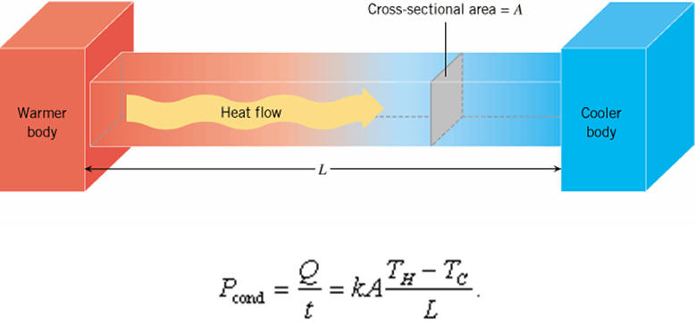
We also need to deploy *Newton's law of cooling*, which states that heat flows from higher T to lower T at the rate proportional to the gradient. Thus the flow of one side can be denoted as
-\kappa h \frac{\partial u}{\partial x}(x+\Delta x,y,t)
Thus the whole square
-\kappa h(\frac{\partial u}{\partial x}(x+\Delta x,y,t)-\frac{\partial u}{\partial x}(x-\Delta x,y,t)\\ +\frac{\partial u}{\partial x}(x,y+\Delta y,t)-\frac{\partial u}{\partial x}(x,y-\Delta y,t))
Transfer by the definition of differentiation, we will get the Time-dependent Heat Equation:
\frac{\sigma}{\kappa}\frac{\partial u}{\partial t}=\frac{\partial^2u}{\partial x^2}+\frac{\partial^2u}{\partial y^2}

2.2 Steady-state heat equation in the disc

If there is no more heat-exchange, the system reaches thermal equilibrium and \partial u/\partial t=0. In this case, the equation reaches the steady-state.
0=\frac{\partial^2u}{\partial x^2}+\frac{\partial^2u}{\partial y^2}
by Laplacian, we can transfer the expression into
\Delta u=0
Our target is to solve the equation on a specific plane or using polar coordinate.
D={(x,y)\in \R^2:x^2+y^2<1}={(r,\theta):r<1}
Rewrite the expression with polar coordinate
\Delta u=\frac{\partial^2u}{\partial r^2}+\frac{1}{r}\frac{\partial u}{\partial r}+\frac{1}{r^2}\frac{\partial^2u}{\partial\theta^2}=0
Or we multiply both sides by r^2
r^2\frac{\partial^2u}{\partial r^2}+r\frac{\partial u}{\partial r}=-\frac{\partial^2u}{\partial\theta^2}
With the aid of separation of variables used in the standing waves and set u(r,\theta)=F(r)G(\theta), we have
\frac{r^2F''(r)+rF'(r)}{F(r)}=-\frac{G''(\theta)}{G(\theta)}
We then set they both equal to \lambda
\begin{cases}
G''(\theta)+\lambda G(\theta)=0 \\
r^2F''(r)+rF'(r)-\lambda F(r)=0
\end{cases}
These equations are much similar to what we have derived in standing waves. We can then use Fourier analysis to solve this problem.

Now! We start our trip to the FOURIER ANALYSIS!